Stats with Silas

Silas Underhill


| Current | Coming Month | |||
| Event | $\bar{x}$ | $P(H)$ | $P(H|E)$ | Protection |
| Erosion | - | - | ||
| Drought | - | |||
| Pests | ||||
| Disease | ||||
| Weeds | ||||
| Gloom | - | |||
| Soil Quality | Counts | Vibe | Counts |
|---|---|---|---|
| Superior | Playful | ||
| Great | Energized | ||
| Good | Seeking | ||
| Average | Thoughtful | ||
| Poor | Unsatisfied | ||
| Terrible | Worried | ||
| Fey |
(Scroll Down to View)

| P(H) | |
| P(E+) | |
| P(E+|H) | |
| P(H|E+) |
| P(H) | |
| P(E-) | |
| P(E-|H) | |
| P(H|E-) |
Village Market
Welcome to StatFarm
by
Jerry Fisher, PhD
Jerry Fisher, PhD
StatFarm is a statistical simulation game where you can review key statistical concepts and grow the best virtual tomatoes you can!
How to Play:
Game Introduction (1/45)
Please enter your name in the textbox. Or you can just leave it blank and go by 'Player'.
The game takes anywhere from 20 - 50 minutes, depending on time spent with the tutorials.
The game takes anywhere from 20 - 50 minutes, depending on time spent with the tutorials.
Welcome to StatFarm! My name’s Silas Underhill. I’m the lead horticulturist around here.
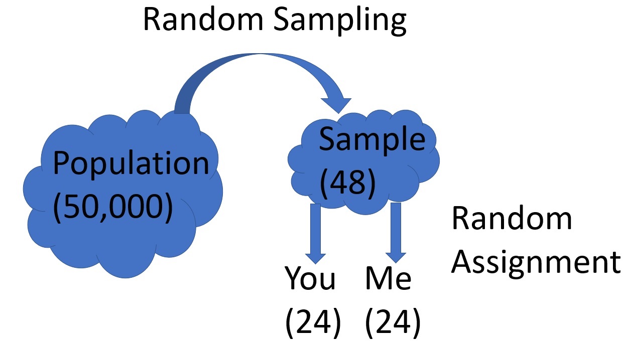
Are you here for the tomato gardener position? Each summer, we grow around 50,000 tomato plants
on the farm, and we're looking for an experienced hand to make sure they grow healthy and right.
Before we can entrust you with the entire population of 50,000 plants, you must first prove yourself by beating me in a growing contest!
Before we can entrust you with the entire population of 50,000 plants, you must first prove yourself by beating me in a growing contest!
This contest will be modest-- it will just involve 48 tomato
plants that we randomly sample from our population of 50,000. We'll randomly assign 24 of these plants
to your care and 24 to my care.
In the following pages, I will discuss the flow of game-- but you can always skip the intro and start right away. Sometimes the best way to learn is to do!
In the following pages, I will discuss the flow of game-- but you can always skip the intro and start right away. Sometimes the best way to learn is to do!
There are two open plots that we will use. I’ll take one plot for my 24 tomatoes, and you take the other
plot for your 24 tomatoes. The two plots are roughly equivalent in terms of the sunshine, rainfall,
and exposure to harm. There should be no statistically significant
differences if we compare measurements between your crop and mine.
We want our plots to be similar in all respects except for the gardener (you or me).
In other words, Gardener is our Independent Variable. Our contest will determine
whether your 24 plants do statistically significantly better than my 24 plants by the end of the growing season.
How do we determine whether your plants do statistically significantly better than mine? We can do this by
comparing yields. In other words, Yield is our Dependent Variable. If your 24 plants yield
a Greater number of tomatoes than my 24 plants, you win.
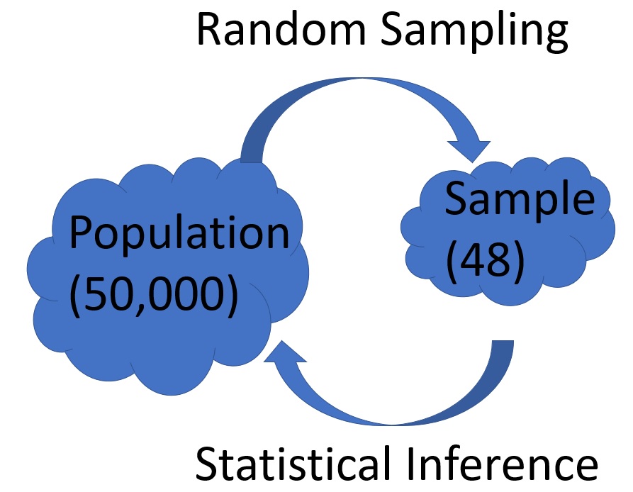
Now, although our contest just involves 48 sprouts, we will be making inferences from the results
about how we’d compare across our population of 50,000.
In essence, if you can distinguish your gardening skills from mine with this sample,
we will infer that this difference would hold with respect to our population.
Let’s now talk briefly about the variables that we will measure in our contest.
These measurements will make up our full (or raw) data.
From the raw data, we can estimate things, such as central tendency, standard deviation,
and group differences.
You can download a CSV file of the raw data at any time in the game. You are encouraged to play around and analyze these data with your favorite statistical analysis program.
You can download a CSV file of the raw data at any time in the game. You are encouraged to play around and analyze these data with your favorite statistical analysis program.
You can scroll down to see the raw data.
Let's talk about each column.
The Gardener is simply you or I. In an experimental context, we could think of this as the independent variable. We want to know if this variable will affect the Yield (the dependent variable) of tomatoes you grow.
The Gardener is simply you or I. In an experimental context, we could think of this as the independent variable. We want to know if this variable will affect the Yield (the dependent variable) of tomatoes you grow.
Gardener and Yield are our two key variables.
But we will also measure other variables that are relevant and explanatory.
Some of these variables may be influenced
by the Gardener's actions, but other variables may be out of the Gardener's hands.
The Plant # column is the plant number. Each of us will have 24 plants.
The Health column is a general assessment of health. It is an ordinal measure that ranks health as "Fantastic", "Great", "Good", "Average", "Poor", or "Moribund"
The Height column is the height of the plant in inches. This is a quantitative variable.
The Health column is a general assessment of health. It is an ordinal measure that ranks health as "Fantastic", "Great", "Good", "Average", "Poor", or "Moribund"
The Height column is the height of the plant in inches. This is a quantitative variable.
The Vibe column is an odd one. Some farmers simply ignore this measurement, while others follow it
closely. In general, people agree that a plant's vibes can have broad effects over its growth, fortitude,
and fruitfulness.
For this measurement, each plant will be categorized as “Seeking”, “Playful”, “Energized”, “Thoughtful”, “Worried”, “Unsatisfied”, or “Fey”.
For this measurement, each plant will be categorized as “Seeking”, “Playful”, “Energized”, “Thoughtful”, “Worried”, “Unsatisfied”, or “Fey”.
Sun is the average daily number of minutes of full sun the plant receives that month. It is a quantitative variable.
Rainfall is measured in inches per week. It is quantitative. Now keep in mind that rainfall is just one way in which a plant can receive water.
Rainfall is measured in inches per week. It is quantitative. Now keep in mind that rainfall is just one way in which a plant can receive water.
When the rainfall is too little, you should take the necessary steps to keep your plants hydrated.
This brings us to the next measure, which is Hydration. This is a simple categorical variable that is either “sufficient” or “insufficient”.
This brings us to the next measure, which is Hydration. This is a simple categorical variable that is either “sufficient” or “insufficient”.
Soil is the quality of the soil. This is an ordinal measurement whose values are ranked from "Superior",
“Great”, “Good”, “Average”, “Poor”, or “Terrible”.
Weeds is the proportion of the plant’s surrounding soil that is occupied by weeds. Its value can range from 0 to 1. You’ll want to keep the weeds down.
Weeds is the proportion of the plant’s surrounding soil that is occupied by weeds. Its value can range from 0 to 1. You’ll want to keep the weeds down.
Pests is the proportion of the plant that is infested with pests. Its value can range from 0 to 1.
You can take preventative or corrective measures to control pest levels.
Disease is the proportion of the plant that is infected with disease. Its value can range from 0 to 1.
Similar to pests, you can take preventative or corrective measures to control disease.
Try to avoid widespread infection of your crop.
Finally, our critical variable of interest. Yield is a plant’s total harvest of tomatoes in pounds.
This quantitative variable will start accumulating around July.
We will compare Yield at the end of the season to see whether the Gardener made a difference.
While the raw data are comprehensive, they are quite a bit of information to
take in and interpret all at once. It is often useful to summarize the raw data in values
that reflect central tendency, variability, and frequency of occurrence. Hence we have the descriptives
table.
For quantitative variables, such as Height, we can summarize the data with the mean (or Average)
and standard deviation (measure of variability). For ordinal and categorical variables, we can
count their frequency of occurrence.
Next, let's look at the game board, the various events that could occur in the coming month, and
ways in which to prepare for them.
If you look below, you will find the game board for May. The little plant icon is where you are in
the game board.
To the right, you can see some coins, a crude die, and some buttons. You will earn coins at various
points on the game board, which can be spent on protection, recovery, and other services.
In may, the first three columns (t test, Chi-Sq, and Race) have only one outcome
(Height, Vibe, Linear). Once you get to the fourth column (Forecasting), you will start rolling
the die, which will determine the cell that is activated for that column.
To the left, you will see a table with the six events. This table provides
information about your current crop, how likely an event will occur in the coming month,
and how protected the crop is.
Let's fill in the first column, the $\bar{x}$ column, which provides your plot's
current mean (or Average) level of pests, disease, and weeds. We will discuss the
other columns later.
Looking back at the game board below, you can see that the plant is
currently at the first column on the left, which involves a t Test.
This t test column is part of a general class of columns for statistical tests.
For these, you will review the formula, perform the test on the relevant variable,
and try to earn some coins.
The t Test is used to make
inferences about group (or condition) differences in the population. We can do t Tests on
quantitative measurements. The game begins with a t Test for Height.
After finishing the t Test, you will move to another statistical test column,
which involves a Chi-Sq test
(Goodness of fit). We will do this test on the categorical variable of Vibe.
Next, you will arrive at a Racing event column, where you can earn
coins by guessing which particular parameters in a function will allow it
to reach y = 100 first (as x increases).
Following this, you will arrive at a Forecasting column. Here, you will consider the probabilities
of adverse events occurring in the coming month. Let's discuss these specific events.
An Erosion event is a sudden and sharp degredation of your plot's soil quality.
There is no protection for this, but supplemental fertilization can offset its effects.
Keep in mind that soil quality can also gradually weaken over time even without an erosion event.
Droughts are a severe and prolonged lack of rain for the coming month. Insufficent hydration can
severely impact your plant's health. Therefore, a wise gardener arranges supplemental watering if
there is any sign of a coming drought.
Pest, Disease, and Weed outbreaks are sharp increases in their levels (far sharper than their
natural accumulation). Successful gardeners forecast wisely and arrange sufficient protection
if needs be. Curative services are also available, but 'an ounce of prevention...'
A Gloom is a distinct period where heavy clouds block the sunlight, leading to
slowed plant growth and souring vibes (at the beginning of stat modification for the month). Although nothing can be done
about a Gloom's effect on sunlight,
there is protection for a plant's vibes.
Any or all of these adverse events could occur in the coming month.
Maybe your luck (and Silas's luck) will hold, and nothing will happen.
Then again, maybe your luck won't hold. The wise farmer assesses probabilities
and plans accordingly.
In the table to the left, the $P(H)$ column provides the StatFarm Almanac's
probability of any of the six events happening based on prior experience.
At the start of each new month, you will be given these priors. Let's fill it in for May.
The prior probability is useful for forecasting, but it can be updated by new evidence.
This update is the posterior probability ($P(H|E)$), which is more accurate. During forecasting,
you will search for such evidence.
When you arrive at a Market column, you will have a chance to spend your coins on protective, healing,
and other services for your crop. You will have a chance to visit three Market columns in
each month's game board. Make sure to spend most of your coins each month because you can only bring
one coin into a new month.
The General store carries a variety of services-- but they are rather
pricey for their quality. Burk is the owner, and he's opened stores all throughout the marketplace.
The Recovery and Protection stores specialize in their respective services. The Recovery store is owned
by hobbits, and Tim Silver runs the protection store.
Finally, there is the Special store. This is store is one of a kind and has some excellent products for
those lucky enough to find it.
Once you get through the game board, the new month will commence. You will then see if any of the
adverse events occurred that month. You will also lose all of your remaining coins except one to taxes.
The coin you will keep will be of the highest value. Also, at the end of the month,
you will get updated data.
And this brings us to the end of the Introduction. Of course, to really learn the game, you just have
to play it a few times. Good luck!
Wave 1: May
The month of May has come and your sprouts are eager to reach for the sun!
| Player | Silas | |
| Yield (sum) |
Wave 1: May
May starts with a t test of height. Click
continue on the right.
t Test
We'll start our contest with a t test of Height. We want to make sure our sprouts are
starting on more-or-less equal footing.
Click 'See Tutorial' for a tutorial on t tests. Otherwise, click on 'Continue Game'.
Click 'See Tutorial' for a tutorial on t tests. Otherwise, click on 'Continue Game'.
t Test Tutorial
Hello. For this tutorial, we will review our raw data, descriptives, and the Independent Samples
t test.
Our first set of measurements just came in.
You can examine them below in the raw data table.
There are 48 rows for the 48 plants we sampled from our population of 50,000 at the farm.
The Gardener column specifies which 24 plants are yours and which 24 plants are mine.
Among the measurements, you'll notice some are quantitative (e.g., height), and
others are categorical (e.g., vibe) or ordinal (e.g., health).
We can summarize the raw data in the descriptive below.
First, you will see the mean ($\bar{x}$) and
standard deviation ($s$) of the quantitative variables in our raw data.
Below that, you can see the counts of the categorical and ordinal variables.
In setting up our contest, we were careful to keep the conditions of the two plots
as similar as possible. So, it is likely that the mean scores for quantitative
variables such as sunlight and rainfall will not be statistically significantly different.
Likewise, we were careful about randomly sampling 48 sprouts from the population of 50,000
and randomly assigning these sprouts to either you or me.
As such, our mean plant heights should not differ much at this point in the contest.
We will test for this.
The formula to calculate the mean ($\bar{x}$) of your sample is:
$$ \bar{x} = \frac{∑x_i} {n} $$
where:
- $x_i$ is each specific value of that set that is indexed by i
- $n$ is the number of values of that set.
Let's calculate the mean height of your 24 sprouts.
The individual scores can be seen on the right (or down below in the raw data table).
In the numerator, we sum up each of these 24 scores. The denominator is simply the number of scores.
Your plot's mean plant height score is
and my plot's mean is
The formula for Standard Deviation ($s$) is:
$$ s = \sqrt{ \frac{∑(x_i-\bar{x})^2} {n-1}} $$
where:
- $x_i$ is each specific value of that set that is indexed by i
- $\bar{x}$ is the mean score of the set
- $n$ is the number of values of that set.
Let's calculate the standard deviation of the height of your 24 sprouts.
In the numerator, we sum up each of the squared differences between a plant and the mean
($\bar{x}$ = .)
In the denominator, we have $n-1$ (Note that sometimes people simply use $n$ instead of $n-1$, but we
won't get into the details of that here).
Your plot's plant height standard deviation is
and my plot's height standard deviation is
As stated earlier,
There are different t tests (independent; dependent) that can be used depending
on the research design. In any case, the t test compares two different groups or
conditions. If you want to compare more than two groups, you will do a different test (e.g., ANOVA).
Here, we will compare your group of 24 plants with my group of 24 plants. Our data are unpaired,
so we will do an independent samples (or unpaired) t test. The dependent samples (or paired)
t test is not discussed in this tutorial.
The formula to calculate an independent samples t test (assuming equal population variance)
is as follows:
$$t = \frac
{\bar{x}_1-\bar{x}_2}
{\sqrt{s^2_p(\frac{1}{n_1}+\frac{1}{n_2})}}$$
where:
- $\bar{x}_1$ is the mean height for your plot
- $\bar{x}_2$ is the mean height for my plot
- $s^2_p$ is the pooled variance (Note that variance is the standard deviation squared)
- $n_1$ is the number of plants in your plot
- $n_2$ is the number of plants in my plot
$$t = \frac
{\bar{x}_1-\bar{x}_2}
{\sqrt{s^2_p(\frac{1}{n_1}+\frac{1}{n_2})}}$$
Looking at the numerator, you can see that we are comparing the means ($\bar{x}$) between your group and my group (it doesn't matter
who is $\bar{x}_1$ and who is $\bar{x}_2$).
Because the t test compares means, it is used to assess group differences between quantitative variables.
Because the t test compares means, it is used to assess group differences between quantitative variables.
It's important to note that the t test involves certain assumptions about the data.
Assumptions:
(All the data here at StatFarm are simulated such that the assumptions are safe)
Assumptions:
- The sample (i.e., the 48 randomly-selected sprouts for our contest) is representative of the population (i.e., the 50,000 plants at StatFarm)
- The data generally follow a normal distribution
- The variance of the two groups is equal
(All the data here at StatFarm are simulated such that the assumptions are safe)
Also, it is important to note that the t test is used within the logic of hypothesis testing.
We use the t test on sample data to draw conclusions about the population.
As part of this, we make a null hypothesis about the population.
The t test will allow you to adjudicate whether you can reject this null hypothesis or not.
Near the end of the contest, we will discuss hypothesis testing in more detail.
Near the end of the contest, we will discuss hypothesis testing in more detail.
Let's calculate the t statistic to compare our plant heights.
Here, for legibility, we are rounding off numbers. As such, the
precise t-statistic value we come up with will be slightly different
from what statistical software will yield.
Here, I am forsaking legibility in order to show you the unrounded values. The
t-statistic derived here is consistent with what you will find using software.
Essentially, we are using the t-test here to examine whether our contest
is fair in terms of the starting plant height. Our assumption here is of a fair contest in terms of height.
Formally, this assumption is that your population mean height is the same as mine.
The t-test allows us to determine whether we can reject this assumption or not.
To interpret our t-statistic, we will have to take into account the degrees of freedom (df)
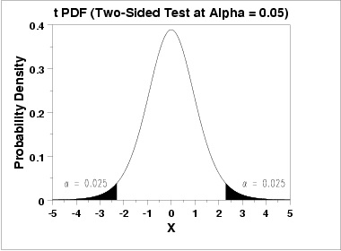
and the subsequent t-critical value. For this comparison, there are 46 degrees of freedom,
and the t-critical value (two-tailed; alpha .05) is 2.01.
If you look to the right, you can see a figure depicting a t distribution. The shaded areas represent the area of the distribution that exceed our t critical value. They are small areas on the tail ends of the distribution.
If you look to the right, you can see a figure depicting a t distribution. The shaded areas represent the area of the distribution that exceed our t critical value. They are small areas on the tail ends of the distribution.
If our t-statistic (absolute value) exceeds the t-crit value, we can conclude that
there is a statistically significant difference between our starting plant heights (and therefore our contest is
not completely fair). We can make this conclusion because, if we assume that we are starting the
contest with plants of equal height, the probability that we would find such a difference in our data
(such that it exceeds the t critical value) is 5% or less.
The term 'p value' represents the probability of obtaining the results that we observe
in our data if the null hypothesis is true. Our null hypothesis is of a fair contest in terms of
starting plant height. If the mean heights between our two groups differ largely, the p-value will be
small. A p value of less than .05 would mean that it is very unlikely
to see the data we see if our null hypothesis is true (so we should reject this null hypothesis).
Let's now compare if our t-statistic (absolute value) exceeds the t-critical value,
and whether we can conclude a statistically significant difference.
t-crit: 2.01
And this concludes our t test tutorial.
Independent Samples t Test
$$t = \frac
{\bar{x}_1-\bar{x}_2}
{\sqrt{s^2_p(\frac{1}{n_1}+\frac{1}{n_2})}}$$
$\bar{x}_1 - \bar{x}_2$ =
$t = \frac
{\bar{x}_1-\bar{x}_2}
{\sqrt{s^2_p(\frac{1}{n_1}+\frac{1}{n_2})}}$
The t critical value (two-tailed; alpha .05) is 2.01.
Can we conclude a statistically significant difference in Height?
This concludes the May t test.
Chi Sq Test
One of StatFarm's resident farmers, farmer Popinjay, has a hypothesis that the vibes of plants
start out according to a specific frequency. We can do a Chi-Sq test to see if farmer Popinjay
is on the right track.
Chi SQ Tutorial
Greetings. For this tutorial, we will review categorical data and the Chi Sq Goodness of Fit test.
Categorical (or nominal) data, unlike quantitative data, consists of a categories as outcomes (not numbers).
Height is a quantitative varible. If I ask your height (in centimeters), the outcome would be a number (e.g., '170' or '182', etc.).
In contrast, eye color is a categorical variable. If I ask your eye color, the outcome would be a category (e.g., 'green' or 'blue' or 'hazel', etc.)
Height is a quantitative varible. If I ask your height (in centimeters), the outcome would be a number (e.g., '170' or '182', etc.).
In contrast, eye color is a categorical variable. If I ask your eye color, the outcome would be a category (e.g., 'green' or 'blue' or 'hazel', etc.)
For quantitative variables, such as height, you can collect a set of observations
(e.g., sample 24 people) and then calculate the mean score and standard deviation of the set.
For categorical variables, such as eye color, calculating the mean and standard deviation is not possible. However, you can still make sense of the data by counting the frequency of occurrence. For example, if you think that 'green' is the most common eye color, you can test this by counting how many people in the set have green eyes compared to other eye colors.
For categorical variables, such as eye color, calculating the mean and standard deviation is not possible. However, you can still make sense of the data by counting the frequency of occurrence. For example, if you think that 'green' is the most common eye color, you can test this by counting how many people in the set have green eyes compared to other eye colors.
Our measurement of Vibes is a categorical variable. If you look at the descriptives below, you will
see the current counts of your crop's vibes and Silas's crop's vibes.
Now then, allow me to introduce my hypothesis. I posit that the May sprouts at StatFarm follow a
reliable frequency of vibes. You see, when a new sprout enters into life, they know little of the
world and its trials and tribulations. They seek to establish their roots and reach for the sun.
As such, roughly half of all sprouts have a 'seeking' vibe. The other half of sprouts are equally likely
to have an 'energized', 'playful', or 'thoughtful' vibe. I don't believe any new sprouts start of
as 'unsatisfied', 'worried', or 'fey'.
On the right, you will see my expected distribution of vibes if we were to sample 48 sprouts. Now,
I just need the actual data from 48 sprouts to test whether my expected distribution is accurate.
Fortunately, you and Silas have the data from 48 sprouts that were randomly sampled from the population.
I ask that you two kindly share your data.
Now, I understand that you are in a contest with Silas and that you two are interested in differences
between your data. But, for my research question, I don't need to distinguish between your two sets. I
will simply ignore whose crops are whose and just combine your
two sets of 24 observations of plant vibes into one larger set of 48 observations.
You can see these observed data on the right (next to the expected frequencies).
Now, of course, the actual frequency may not match up exactly with the expected frequency. It is likely to differ a little. The question is: do the actual data differ statistically significantly from the expected data?
Now, of course, the actual frequency may not match up exactly with the expected frequency. It is likely to differ a little. The question is: do the actual data differ statistically significantly from the expected data?
The formula for a Chi Sq test of Goodness of Fit is as follows:
$$
{\chi}^2 = ∑\frac{(Obs-Exp)^2}{Exp}
$$
Let's calculate:
$$
{\chi}^2 = ∑\frac{(Obs-Exp)^2}{Exp}
$$
Our ${\chi}^2$ value was
.
We will compare this value to our ${\chi}^2$ critical value (alpha .05; df 3), which is 7.815.
We will compare this value to our ${\chi}^2$ critical value (alpha .05; df 3), which is 7.815.
Chi Square Goodness of Fit Test
$
{\chi}^2 = ∑\frac{(Obs-Exp)^2}{Exp}
$
t Test
We'll start june with
. Click on 'Continue Game'.
Independent Samples t Test
Analysis of Variance (ANOVA)
We'll start July with
. Farmers Noontide and Rainmaker have agreed to share the quantitative data from their crops
for this analysis. You can see their data if you scroll down below. You can see our tutorial on the analysis of variance
(ANOVA) test or just continue the game.
ANOVA Tutorial
- $n_i$ is the number of plants in each group (indexed by $i$)
- $\bar{x}_i$ is the mean score of each group (indexed by $i$)
- $\bar{\bar{x}}$ is the grand mean (of all the groups combined)
- $k$ is the number of groups
- $n_i$ is the number of plants in each group (indexed by $i$)
- $s_{i}^2$ is the variance of each group (indexed by $i$). Note that the variance is the standard deviation squared.
- $n_t$ is the total number of plants (combining all the groups)
- $k$ is the number of groups
Analysis of Variance (ANOVA)
Regression
We'll do a regression of Yield on Height. Click on 'Tutorial' or 'Continue'.
Regression Tutorial
Regression
Bayes Barnyard
Forecasting
Let's talk about forecasting. Bayes Barnyard is a place where we calculate probabilities
of certain adverse events occurring. We will follow Bayes Theorem, which allows us to
take into account prior knowledge and new evidence.
Life can sometimes be tough and uncertain.
The same is for a plot of tomatoes. In the months ahead, nature could throw
some difficult events at your plot and Silas's plot. How you prepare for these
events will go a long way towards your crops height, health, and fruitfulness.
Every month brings a new probability for one or more adverse events to strike.
In forecasting, you will estimate these probabilities based on previous experience and new evidence.
Estimating these probabilities is important because you will likely not have enough time or money
to prepare for every potential event.
Fortunately, you have information at your disposal that can help guide your decision making in
preparing for adverse events.
For instance, at the beginning of each new month, you will get StatFarm almanac's prior probability of each event occurring that month (see the $P(H)$ column in the game board table to the left).
Note that this probability (and all others) change from month to month.
For instance, at the beginning of each new month, you will get StatFarm almanac's prior probability of each event occurring that month (see the $P(H)$ column in the game board table to the left).
Note that this probability (and all others) change from month to month.
While a prior probability ($P(H)$) is a useful piece of information to guide your decision making,
it can be updated if new evidence is observed. For example, you could administer a specific test
that aims at detecting whether an adverse event will occur in the coming month.
The results of this test will serve as evidence.
This updated probability given the evidence is the posterior probability ($P(H|E^+)$). It can be calculated using Bayes Theorem (see right).
This updated probability given the evidence is the posterior probability ($P(H|E^+)$). It can be calculated using Bayes Theorem (see right).
And this concludes our forecasting tutorial.
Sometimes you need to calculate $P(E)$, which you can do with the following formula:
$$P(E) = P(H)P(E|H) + P(¬H)P(E|¬H)$$
Where:
- $P(E)$ is simply the probability of observing the evidence (without taking into account the hypothesis)
- $P(H)$ is simply the probability of the hypothesis (without taking into account evidence)
- $P(E|H)$ is the probability of observing the evidence if the hypothesis is accurate
- $P(¬H)$ is simply the probability of the hypothesis not being accurate
- $P(E|¬H)$ is the probability of observing the evidence if the hypothesis is not accurate
Linear Race
It is time for racing! The current races are between four
functions.
Click 'See Tutorial' for a general tutorial on racing. Otherwise, click on 'Continue Game'.
Click 'See Tutorial' for a general tutorial on racing. Otherwise, click on 'Continue Game'.
Linear Race Tutorial
Let's talk about about racing. Each race involves four contenders that will race across
the x-axis to see which one can first get their y score to 100.
If you run your math right, you can win some nice coins.
Sometimes the four contenders all belong to the same function (e.g., a linear function). But if you come to a Grand race, each contender will be of a different function.
Sometimes the four contenders all belong to the same function (e.g., a linear function). But if you come to a Grand race, each contender will be of a different function.
The four potential functions that a contender could be are:
The parameters $b$ and $m$ will vary for every new race ($m$ specifies the rate of increase;
$b$ is the intercept/scaling factor).
| Linear | $y = m \cdot x+b$ |
| Exponential | $y = b \cdot e^{m \cdot x}$ |
| Power | $y = b \cdot x^m$ |
| Logarithmic | $y = m \cdot ln(x) + b $ |
Here are the prizes:
- A gold coin
- Pick the first place winner of a Grand Race.
- A silver coin
- Pick the first place winner of a Linear, Power, Exp, or Log race.
- Pick the second place finisher of a Grand Race.
- A bronze coin
- Pick the second place finisher of a Linear, Power, Exp, or Log race.
- Pick the third place finisher of a Grand Race.
Each time you land on a race column, you can attend two races.
That's all there is to it. You'll get the hang of racing rather quickly.
That's all there is to it. You'll get the hang of racing rather quickly.
You have remaining. Here are the functions' values this race:
The new month brings ...
| $P(H)$ | $P(H|E)$ | Protection | Occurrence | Severity | |
| Erosion | - | ||||
| Drought | |||||
| Pests | |||||
| Disease | |||||
| Weeds | |||||
| Gloom |
| Silas | ||
| Sum Total Yield |
About
- StatFarm is a free, interactive game/lesson that simulates data for a growing contest. It is intended to provide users who are new to statistics a familiarity with organizing data, summarizing data, and drawing statistical inferences. It’s also intended to be fun!
- This game was written with the perspective that learning is most effective when it is engaging, interactive, and rooted in real-world examples. Throughout the game, the user will track data and probabilities for events in order to properly tend to their simulated crop.
- The data consist of simulated measurements of quantitative, ordinal, and categorical variables. The initial quantitative data are simulated according to a random normal distribution, and data modification (e.g., due to events) is also normally distributed.
- As the game progresses, the user will have the option to review various statistical procedures, such as the independent samples t-test, Chi-Sq, analysis of variance (ANOVA), and regression. These statistical tests will be performed on the simulated data. Additionally, the user will be introduced to Bayes Theorem as part of predicting upcoming events.
- At any point in the game, the user can download their data in .csv format. These data can be easily read into statistical software such as Excel, SPSS, SAS, R. As such, this game can also be used in a classroom context (see Lesson Plans below).
- This game was also written with the spirit that education should be accessible for everybody. As such, this game is free and available to everybody.
Lesson Plans
- (coming soon)
| Test Result | Event | $P(H)$ | $P(E)$ | $P(E|H)$ | $P(H|E)$ |
|---|---|---|---|---|---|
| Erosion | |||||
| Drought | |||||
| Pests | |||||
| Disease | |||||
| Weeds | |||||
| Gloom |
(Don't click browser back button. To leave, click 'Leave' below.)
1 Gold
- Full (5% Protection and Removal)
- Pest and Disease Protection (8%)
- Pest and Disease Removal (6%)
- Weed and Drought Protection (8%)
- Weed Protection and Removal (7%)
- Gloom Protection (16%) and Vibe Change (Plants that are Fey, Worried, or Unsatisfied have 50% chance of improvement)
- Pest and Disease Protection (4%)
- Pest and Disease Removal (3%)
- Weed and Drought Protection (4%)
- Weed Protection and Removal (3%)
- Gloom Protection (8%)
- Fertilizer (Soil quality increases 2 levels for 2 plants)
(Don't click browser back button. To leave, click 'Leave' below.)
1 Gold
- Comprehensive (30% Protection for all)
- Drought Protection (30%)
- Pest Protection (30%)
- Disease Protection (30%)
- Weed Protection (30%)
- Gloom Protection (40%)
- Drought Protection (15%)
- Pest Protection (15%)
- Disease Protection (15%)
- Weed Protection (15%)
- Gloom Protection (20%)
- Lottery ticket (10% chance winning Gold, 25% chance winning Silver)
(Don't click browser back button. To leave, click 'Leave' below.)
1 Gold
- Comprehensive (20% Removal for all)
- Pest Removal (20%)
- Disease Removal (20%)
- Weed Removal (20%)
- Pest, Disease, and Weed Removal (7%)
- Fertilizer (Soil quality increases 1 level for 12 plants)
- Pest Removal (10%)
- Disease Removal (10%)
- Weed Removal (10%)
- Pest, Disease, and Weed Removal (3%)
- Fertilizer (Soil quality increases 1 level for 6 plants)
- Gloom Protection (10%) and Vibe Change (Plants that are Fey, Worried, or Unsatisfied have 50% chance of improvement)
(Don't click browser back button. To leave, click 'Leave' below.)
1 Gold
- Full Protection and Removal (20%)
- Full Protection (17%)
- Full Removal (15%)
- Drought Protection (40%)
- Pest/Disease/Weed Removal and Protection (7%)
- Fertilizer (Soil increases 2 levels for 4 plants; 1 level for another 8 plants)
- Full Protection (6%)
- Full Removal (5%)
- Drought Protection (20%)
- Pest/Disease/Weed Removal and Protection (3%)
- Fertilizer (Soil increases 2 levels for 2 plants; 1 level for another 4 plants)
- Gloom Protection (30%) and Vibe Change (Plants that are Fey, Worried, or Unsatisfied have 100% chance of improvement)

| Height | |||
| 1 | 13 | ||
| 2 | 14 | ||
| 3 | 15 | ||
| 4 | 16 | ||
| 5 | 17 | ||
| 6 | 18 | ||
| 7 | 19 | ||
| 8 | 20 | ||
| 9 | 21 | ||
| 10 | 22 | ||
| 11 | 23 | ||
| 12 | 24 | ||
| Gardener | $n$ | $\bar{x}$ | $s$ |
| 24 | |||
| Silas | 24 | ||
| Noontide | 24 | ||
| Rainmaker | 24 | ||
| Grand | |||
 |
 |
 |
| 0 | 0 | 0 |

| Vibes | Expected Counts | Observed Counts |
|---|---|---|
| Playful | 8 | |
| Energized | 8 | |
| Seeking | 24 | |
| Thoughtful | 8 |
Bayes Theorem:
$$P(H|E^+) = \frac{P(E^+|H)P(H)}{P(E^+)}$$- $P(H)$ is simply the probability of the hypothesis (e.g., the event occurring) based on prior experience. This is the prior.
- $P(E^+)$ is simply the probability of observing the evidence (e.g., a positive outcome on a test for the event).
- $P(E^+|H)$ is the probability of observing the evidence (e.g., a positive test) if the hypothesis is accurate (e.g., the event indeed occurs). This is the likelihood.
- $P(H|E^+)$ is the probability of your hypothesis (e.g., the event occurring) given certain evidence is observed (e.g., a positive test). This is the posterior, and it is important information for forecasting.
Bayes Theorem:
$$P(H|E^-) = \frac{P(E^-|H)P(H)}{P(E^-)}$$- $P(H)$ is simply the probability of the hypothesis (e.g., the event occurring) based on prior experience. This is the prior.
- $P(E^-)$ is simply the probability of observing the evidence (e.g., a negative outcome on a test for the event).
- $P(E^-|H)$ is the probability of observing the evidence (e.g., a negative test) if the hypothesis is accurate (e.g., the event indeed occurs). This is the likelihood.
- $P(H|E^-)$ is the probability of your hypothesis (e.g., the event occurring) given certain evidence is observed (e.g., a negative test). This is the posterior, and it is important information for forecasting.
Use the descriptives below to enter the numerator of the t statistic formula in textbox. You should enter a value (e.g., 0.04). Remember, we are doing a t test for Height.

Welcome to Burk's General Store. We provide all kinds of goods and services.
Welcome to the Hobbit Recovery Store. We source all our goods and services from the Shire. Our main
services are plant recovery, but we also offer fertilizer and some gloom protection.

Welcome to the Tim Silver's Protection Store. We offer fertilizer, watering, weed barriers and
other services to protect your plant. If you see trouble coming, this is the place to shop.

Welcome to the Special Shop.
| Number | Height ($x$) | Yield ($y$) |
| 1 | ||
| 2 | ||
| 3 | ||
| 4 | ||
| 5 | ||
| 6 | ||
| 7 | ||
| 8 | ||
| 9 | ||
| 10 | ||
| 11 | ||
| 12 | ||
| 13 | ||
| 14 | ||
| 15 | ||
| 16 | ||
| 17 | ||
| 18 | ||
| 19 | ||
| 20 | ||
| 21 | ||
| 22 | ||
| 23 | ||
| 24 | ||
| 25 | ||
| 26 | ||
| 27 | ||
| 28 | ||
| 29 | ||
| 30 | ||
| 31 | ||
| 32 | ||
| 33 | ||
| 34 | ||
| 35 | ||
| 36 | ||
| 37 | ||
| 38 | ||
| 39 | ||
| 40 | ||
| 41 | ||
| 42 | ||
| 43 | ||
| 44 | ||
| 45 | ||
| 46 | ||
| 47 | ||
| 48 |